
Can You Win Everything with A Lottery Ticket?
TL;DR
Recent works have demonstrated that it is possible to obtain sparse networks that are competitive with dense networks. The outperformance of sparse networks have been investigated primarily in terms of test set accuracy. In this post, I will attempt to summarize the paper Can You Win Everything with A Lottery Ticket?[@chencan] which assesses performance of sparse networks across multiple dimensions, datasets and architectures. I discuss related prior work, the proposed dimensions for assessing neural network performance and the important metrics for each dimension. I conclude by highlighting the strengths and limitations of the paper.
Introduction
Neural networks have achieved good performance on a variety of tasks
ranging from image classification to object detection. However a
rigorous notion of good performance still remains an open topic of
research. The difficulty can be partly attributed to the different
perceptions of good performance in different contexts. In the context of
many non-critical industrial applications, simple metrics like high test
set accuracy or lower values of test set loss may seem to be sufficient.
These metrics while simple to compute and easy to study, often do not
give a complete picture of neural network performance. Understanding the
limitations of metrics becomes particularly important in safety critical
applications like self driving vehicles. Robustness of the network
predictions instead of high test accuracy is of paramount importance in
such use cases. Similarly when neural networks are deployed for medical
diagnosis, interpretability and reliability become as relevant as high
test accuracy.
Considering the limitations of simple metrics, different measures of
performance have been proposed in prior works. Recent works have
attempted to incorporate different metrics for dense networks
[@hendrycks2019benchmarking]. However, a thorough evaluation of
different dimensions of performance for sparse networks remains under
studied. In this post, I will review the paper Can You Win Everything with
A Lottery Ticket?[@chencan] to understand the impact of sparsity on
different measures of performance.
In particular, I tried to understand
-
When can we say that a network performs well ?
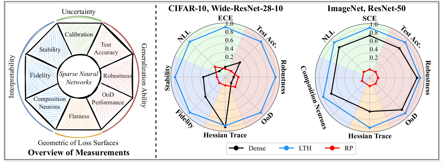
The paper evaluates the performance of sparse networks on multiple dimensions, namely Generalization, Calibration & Reliability, interpretability and geometry of loss landscapes to get a complete picture. A sparse model which out-performs a dense model on all the metrics is considered as LTH-PASS. -
Which aspects of neural networks are more sensitive to sparsification ?
The paper tries to understand if all the metrics are equally impacted by different levels of sparsity and pruning methods. We identify which pruning methods which are less sensitive for each metric. -
Can I use pruning techniques to achieve better performance than dense models ?
It is known that sparse networks can outperform dense networks on accuracy metrics. The paper evaluated if sparse networks can also remain competitive with dense models simultaneously on multiple dimensions.
Prior Work
Evaluation Metrics
Prior works have investigated the performance of sparse networks using test accuracy and adversarial robustness. [@gui2019model], [@ye2019adversarial] have reported that it is possible to obtain good test accuracy and adversarial robustness with compression. Sensitivity to natural image corruptions has also been explored. [@hooker2019compressed] [@hooker2020characterising] have shown that sparse networks are brittle to small changes such as natural image corruptions. Sparse networks have also been observed to amplify the class imbalance more than dense counterparts [@hooker2020characterising]. Some aspects like uncertainty, interpretability and loss landscape are not well studied for sparse networks.
Pruning Techniques
The paper [@chencan] examines the performance across different dimensions as well as different pruning techniques. The paper uses random pruning as a necessary baseline for the sanity check. Among the magnitude pruning techniques, the paper selects One shot Magnitude pruning (OMP) [@han2015deep] in its experiments. In OMP, a portion of Iights with the globally smallest magnitudes are removed. LTH [@frankle2020linear] has recently emerged as a popular technique for pruning. LTH iteratively prune 20% of remaining Iight with the globally smallest magnitudes and rewinds model Iights to the same early training epochs. To reduce training costs, Pruning at initialization (PI) mechanisms have been proposed. PI mechanisms attempt to locate sparse subnetworks at random initialization via certain saliency criterion. SNIP [@lee2018snip], GraSP [@wang2020picking], and SynFlow [@tanaka2020pruning] are considered to studied as part of PI techniques. Dynamic Sparse Training (DST) have recently achieved state of the art results. DST algorithms generally start from a random sparse network and encourage the neural network connectivity and model parameters to evolve simultaneously based on a grow-and-prune strategy. RigL [@evci2020rigging] is considered as an example of DST pruning methods.
Evaluating performance
In the following sections, I discuss the performance of sparse networks across different dimensions. Each dimension is evaluated using multiple metrics. I briefly highlight the important metrics and main takeaways for each dimension.
Generalization
Generalization is studied from following perspectives
-
Test set accuracy: The paper adopts the conventional definition of test set accuracy and evaluate how its variation across different sparsity levels.
-
Out-of-distribution (OoD) performance [@nguyen2015deep]: It has been observed that dense networks are over-confident on out of distribution data [@nguyen2015deep]. ROC-AUC scores on OoD dataset is used to evaluate if over-confidence persists for sparse networks.
-
Natural corruption robustness [@hendrycks2019benchmarking]: Mean Corruption Error (mCE) [@hendrycks2019benchmarking] are used to evaluate the sensitivity of networks to natural image corruptions like noise, blur and Iather.
-
Adversarial robustness: Fast Gradient Sign Method (FSGM) [@goodfellow2014explaining] is used to generate adversarial perturbed image. The test set accuracy is calculated on these adversarial perturbed image.
Figure conventions
The following plots are from the paper [@chencan] and follow the conventions used in the paper. Sparsity levels and metric performance are plotted in X-axis and Y-axis respectively. The sparsity levels are obtained by iteratively pruning with a ratio of 20%, i.e., \((1-0.8^n) \times 100\%\) where \(n\) is the number of pruning rounds. The black dashed lines in each plot denote the performance of Dense model. \(\uparrow\) denotes higher values of the considered metric is better while \(\downarrow\) denotes that lower values are better. Each curve is divided into three regions based on drop in performance. Region I (solid lines) indicates winning tickets and region II denotes degraded subnetworks (dash lines).
Generalization Results

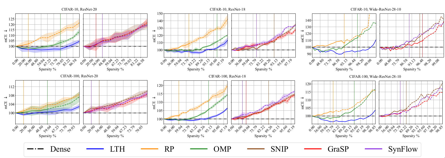
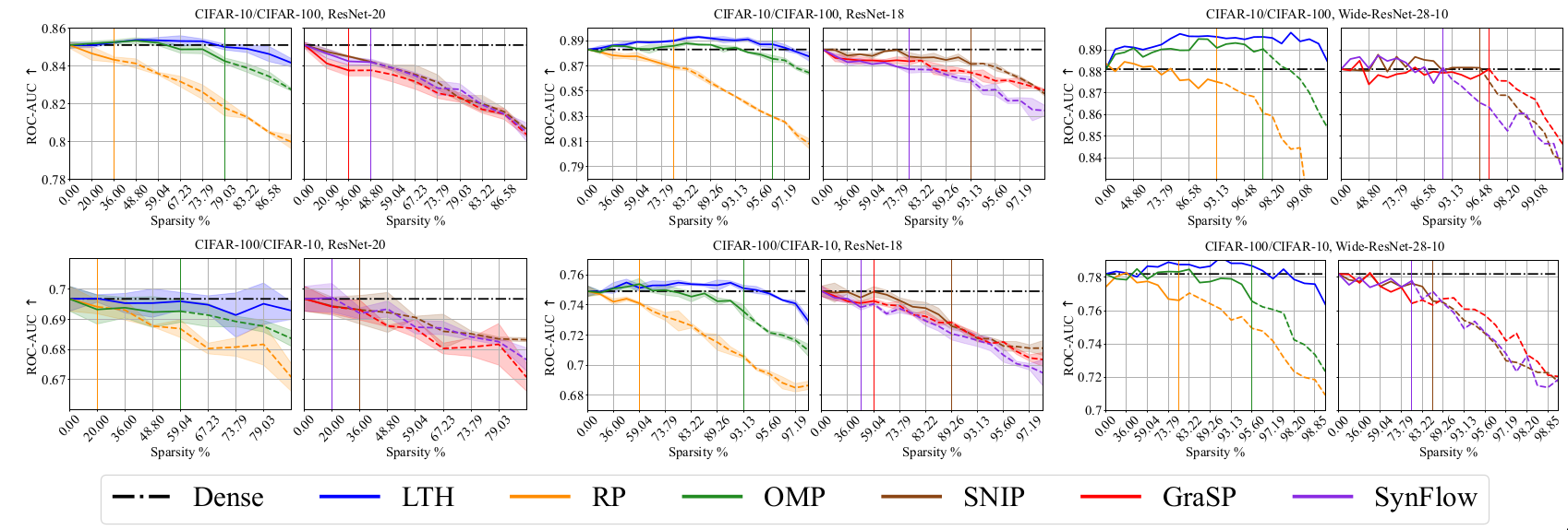
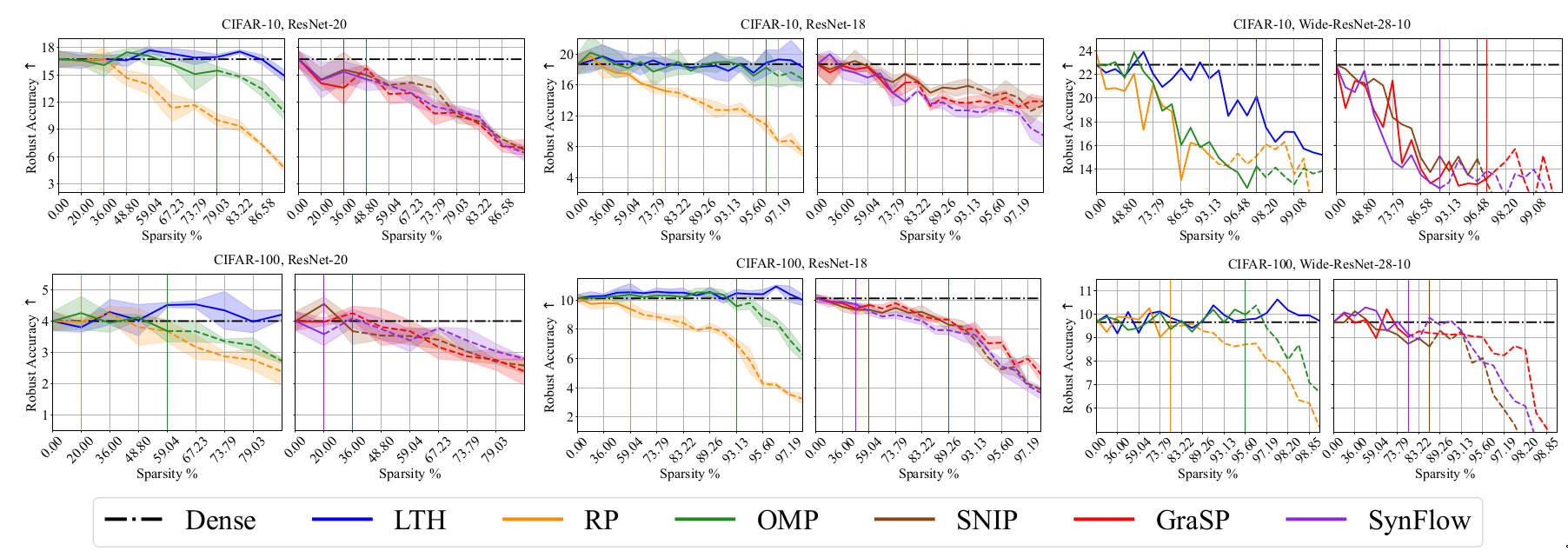
Discussion
The metrics considered along the generalization dimension have been well
studied and generally accepted to have high practical relevance. The
experimental results in the paper help us to evaluate the effect of
sparsity across these metrics. While sparse networks are able to
outperform dense networks, their sensitivity varies for different
metrics. In particular, pruned models seem to be more susceptible to
image corruptions. This resonates with prior results in
[@hooker2020characterising].
The results also help us understand the effect of different pruning
methods, datasets and network architecture. OMP and LTH methods perform
well across most metrics. The sparsity levels at which sparse networks
outperform dense models varies depending on the selected metric. It is
observed that it is harder to obtain good results for C100 than C10. The
larger number of classes in C100 could be a possible explanation.
Over-parameterized models like WR28-10 can achieve good performance at
higher sparsity than R20s.
Calibration and Reliability
It is generally expected that neural network confidence scores reveal the true correctness likelihood. When the predictions are likely to be correct, confidence should be higher and vice-versa. A network which matches this intuition can be said to be well calibrated. Calibration and Reliability are quantitatively studied using the following metrics
-
Expected calibration error (ECE) [@naeini2015obtaining]
The predictions of neural network are partitioned into bins. The discrepancy betIen the accuracy and confidence for each bin is calculated and averaged based on the number of samples in the bin. Let \(n\) denote the total number of samples and \(B_m\) be samples in bin \(m\). Then, \(\text{ECE} = \sum_{m=1}^{M} \frac{|B_m|}{n} |acc(B_m) - conf(B_m)|\) -
Static calibration error (SCE) [@gIon2019reliable] Let \(C\) denote the total number of classes and \(y_i\) denote the label for sample. SCE is calculated as, \(\text{SCE} =\frac{1}{nC} \sum_{c=1}^{C} \sum_{m=1}^{M} |\sum_{i\epsilon B_m} \mathbf{1} (y_i=c) - conf(B_m)|\) While ECE considers only the highest probability, the probabilities of all the classes are considered in SCE.
-
Negative log likelihood (NLL) [@lecun2015deep]
Let \(\hat{p}\) be predicted likelihood for sample \(x\). Then, \(\text{NLL} = -\sum_{(x, y) \sim D_{val}} \text{log}{\hat{p}(y|x)}\)
Lower values of the above considered metrics imply better performance along this dimension.
Calibration and Reliability Results
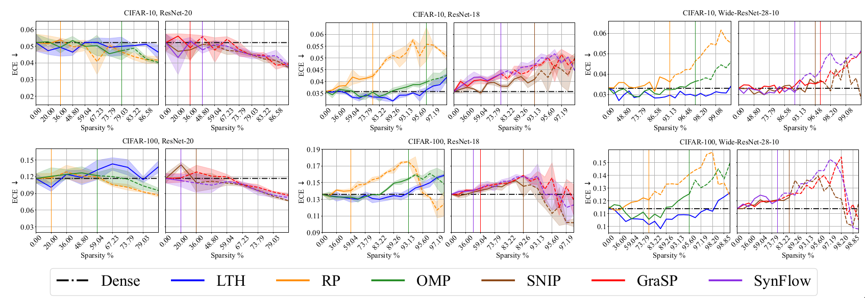
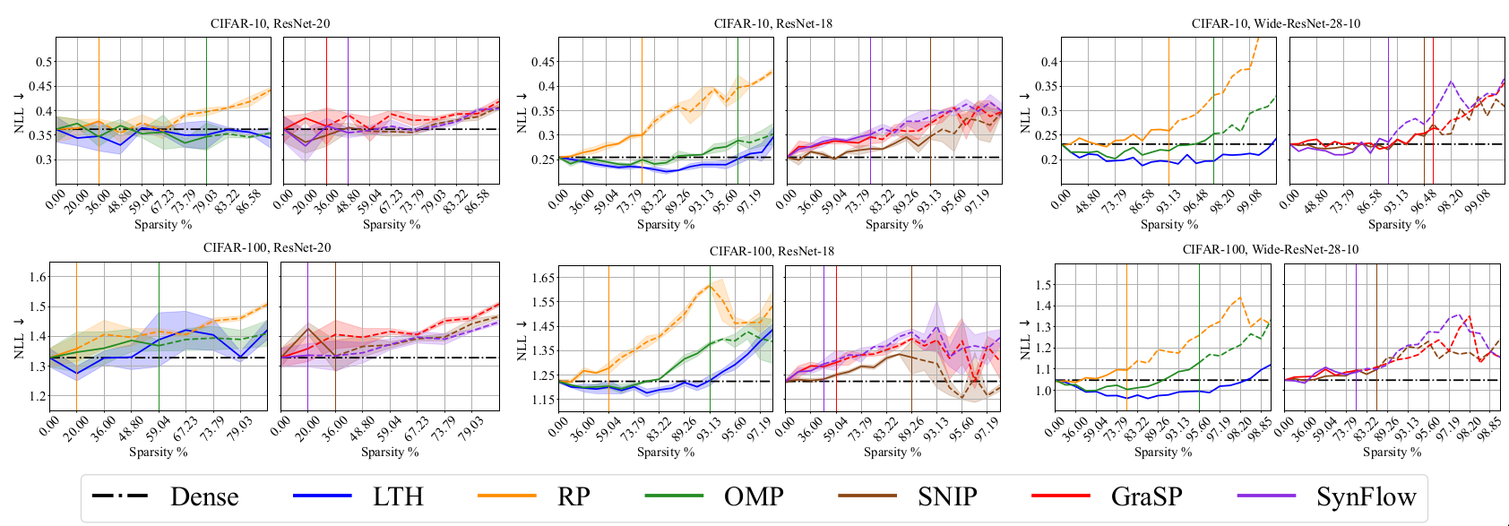
Discussion
The results indicate that it is more difficult to obtain highly sparse
models that outperform dense models along this dimension than
generalization dimension. This observation makes intuitive sense because
the models have been optimized using cross entropy loss which is related
to higher accuracy and not directly connected to calibration &
reliability metrics.
RP and PI methods have superior performance than LTH and OMP along
calibration and reliability dimension. It maybe noted that even though
RP and PI methods outperform along calibration and reliability
dimension, their performance for the generalization dimension is
mediocre.
Interpretability
The predictions of neural networks are sometimes difficult to explain and sensitive to perturbations. If a model’s predictions can be explained from a functional perspective and the predictions are not highly sensitive to slight perturbations then it maybe regarded as more interpretable. The paper considers the following quantitative metrics for evaluation. These metrics try to quantify how the model’s output changes when the input samples are perturbed.
-
Fidelity [@ribeiro2016should]
The fidelity metric helps to quantify how accurately an explainer models the target network. The explainer model is a linear function obtained using regression on the target model’s output. Let \(x\) denote input image and \(f(x)\) be model output. I perturb \(x\) to generate a neighborhood set \(N_x\). I learn linear function \(g_x\) using regression on model output \(f(x)\). Fidelity is defined as \(\mathcal{F} = \mathbb{E}_{x \epsilon D_{val}}[\mathbb{E}_{x' \sim N_x} [{(g(x') - f(x'))}^2)]]\) -
Stability [@plumb2020regularizing] [@alvarez2018towards]
Stability measures the degree to which the explanation changes across points. Let \(g_x\) and \(g_x'\) are linear models trained on neighborhood sets. Let \(e(x, f)\) and \(e(x',f)\) denote the learnt Iights of these linear models. Stability is defined as \(\mathcal{S} = \mathbb{E}_{x \epsilon D_{val}}[\mathbb{E}_{x' \sim N_x} [{(e(x,f) - e(x',f))}^2)]]\)
Lower values of fidelity and stability are desirable. Aside from quantitative metrics like fidelity and stability, the paper also considers the NetDissect procedure to explain the behavior of individual neurons.
Interpretaibility Results
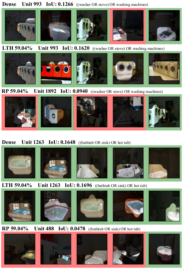
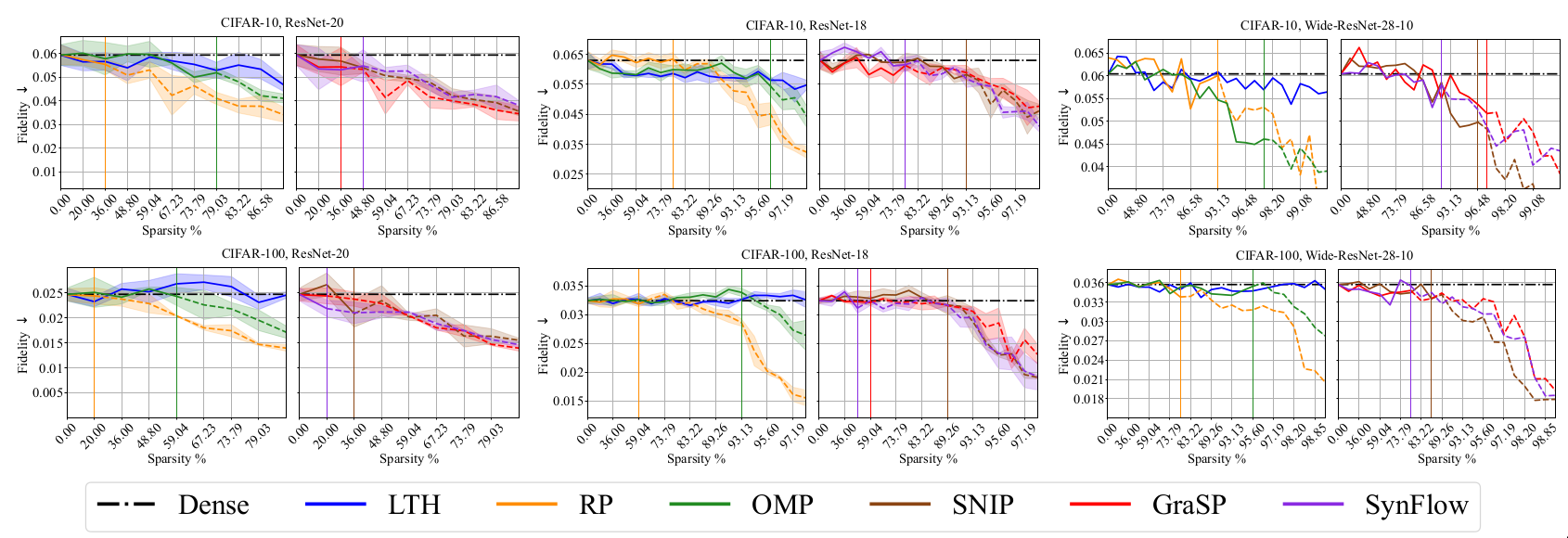
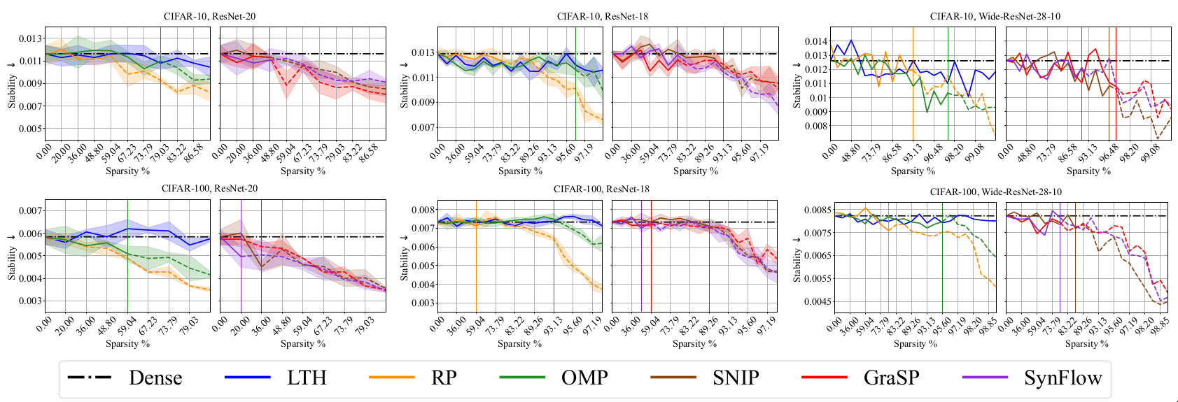
Discussion
Based on the performance on fidelity and stability metrics, RP and PI pruning methods seem to provide more interpretable models. LTH significantly lags behind which could indicate that the representations learnt using LTH are non-linear. Qualitative evaluation using the NetDissect procedure help in providing an intuition regarding the behavior of learnt neurons using LTH. It is shown that neurons in LTH models are interpretable using compositional concepts with the NetDissect procedure.
Geometry of loss landscapes
Prior works [@hochreiter1997flat] [@jiang2019fantastic] have reported that loss landscapes of well-generalizing models are relatively “flat” with respect to model Iights. The works of [@wu2020revisiting] [@moosavi2019robustness] have shown that a flatter adversarial loss landscape with respect to model inputs improves the robustness generalization. To consider both kinds of generalization, the flatness of geometry of loss landscape using the Hessian of objective function with respect to the model Iights and input samples is studied in the paper.
Geometry of loss landscapes
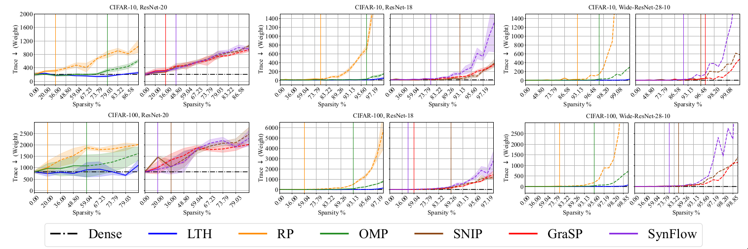
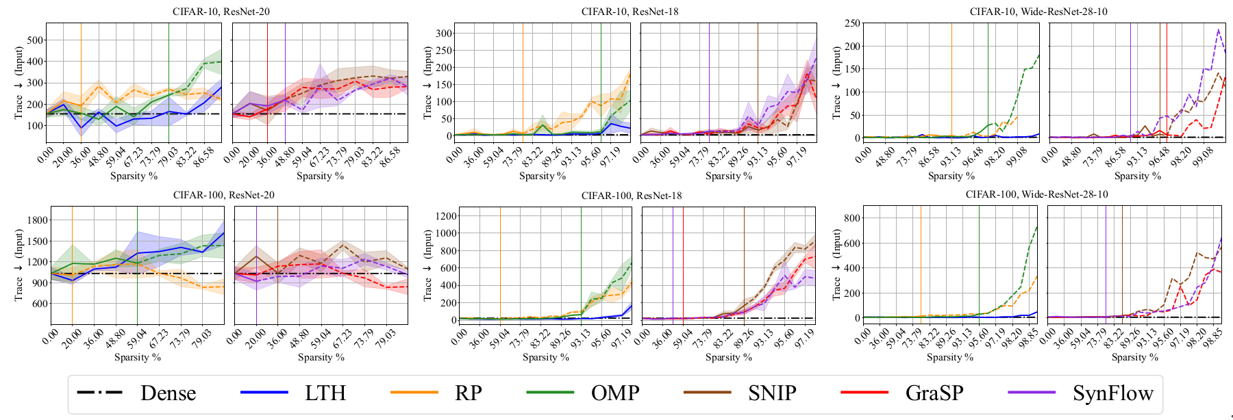
Discussion
Results indicate that the geometry of loss landscapes obtained using different
pruning methods is affected by the architecture and dataset. PI methods
like GraSP, SNIP and SynFlow underperformed on CIFAR-10 for all the
architectures (R18, R20, WR28) while LTH remains competitive with the
dense model performance.
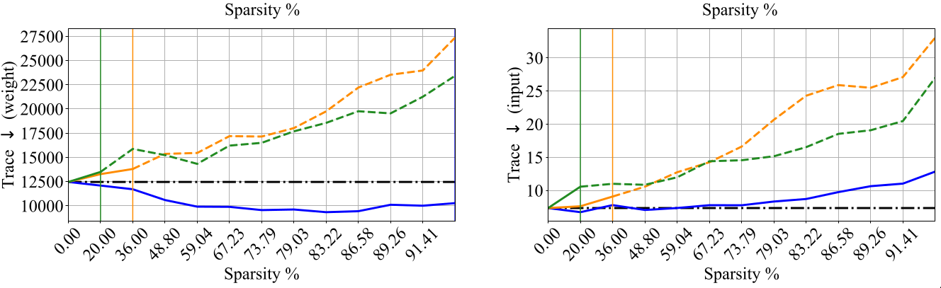
Among the considered pruning techniques, RigL underperformed on this
metric for all the datasets (C10, C100 and ImageNet) for Resnet-50
architecture. Using LTH method on Resnet-50, it is possible to obtain
relatively flat sparse models on all the datasets. PI methods like GraSP
underperform for the Resnet-50 architecture.
Discussion
Strengths
The paper provides a framework to assess the performance of a sparse neural networks on multiple dimensions. Consideration of multiple dimensions helped us to better understand the advantages and limitations of different pruning methods. The experiments in the paper are comprehensive. The paper considers diverse datasets (CIFAR-10, CIFAR-100 and ImageNet) and multiple model architectures (Resnet, Wide Resnet, VGG) in its experiments. To get a good coverage of different pruning techniques, seven different methods are considered. Aside from standard pruning methods like OMP and LTH, pruning at initialization schemes and dynamic sparse training methods have also been selected.
Limitations
Although the paper’s experiments are extensive, results are missing for few metrics. I highlight some of the missing results here
-
Fidelity and stability are discussed as important measures of interpretability. However, fidelity and stability not considered in the ImageNet results.
-
Some metrics (namely SCE, Iight/Input Flatness) are introduced but not evaluated for all the settings.
-
RigL results are missing for CIFAR-10/100 dataset for different sparsity levels.
All the pruning methods considered in the paper perform unstructured
pruning. Recent works [@shen2022prune] have shown that it is possible to
obtain highly sparse models with structural sparsity. An evaluation of
structured pruning techniques on the proposed dimensions would have been
useful to better understand their performance.
The paper considers multiple metrics to assess performance along
different performance dimension. A more detailed discussion about the
motivation for selecting each metric would have been useful. The
advantages and limitation of the considered metrics could also have been
highlighted.
Conclusion
Sparse networks are immensely important from a practical perspective.
The results in the paper help empirically establish that it is possible
to obtain a sparse sub-network that performs better than dense network
across multiple dimensions. Competitive performance on different
datasets and architecture helps substantiate the wide applicability of
the results.
Among the considered methods, LTH remains competitive across most of the
performance dimensions. Some techniques (for instance RigL) lag behind
on certain metrics (geometry of loss landscapes). Future works may
attempt to investigate the reasons for under-performance of the
considered methods on specific dimensions.
References
Alvarez Melis, David, and Tommi Jaakkola. 2018. “Towards Robust Interpretability with Self-Explaining Neural Networks.” Advances in Neural Information Processing Systems 31.
Chen, Tianlong, Zhenyu Zhang, Jun Wu, Randy Huang, Sijia Liu, Shiyu Chang, and Zhangyang Wang. n.d. “Can You Win Everything with a Lottery Ticket?” Transactions of Machine Learning Research.
Evci, Utku, Trevor Gale, Jacob Menick, Pablo Samuel Castro, and Erich Elsen. 2020. “Rigging the Lottery: Making All Tickets Winners.” In International Conference on Machine Learning, 2943–52. PMLR.
Frankle, Jonathan, Gintare Karolina Dziugaite, Daniel Roy, and Michael Carbin. 2020. “Linear Mode Connectivity and the Lottery Ticket Hypothesis.” In International Conference on Machine Learning, 3259–69. PMLR.
Goodfellow, Ian J, Jonathon Shlens, and Christian Szegedy. 2014. “Explaining and Harnessing Adversarial Examples.” arXiv Preprint arXiv:1412.6572.
Gui, Shupeng, Haotao Wang, Haichuan Yang, Chen Yu, Zhangyang Wang, and Ji Liu. 2019. “Model Compression with Adversarial Robustness: A Unified Optimization Framework.” Advances in Neural Information Processing Systems 32.
GIon, Hyukjun, and Hao Yu. 2019. “How Reliable Is Your Reliability Diagram?” Pattern Recognition Letters 125: 687–93.
Han, Song, Huizi Mao, and William J Dally. 2015. “Deep Compression: Compressing Deep Neural Networks with Pruning, Trained Quantization and Huffman Coding.” arXiv Preprint arXiv:1510.00149.
Hendrycks, Dan, and Thomas Dietterich. 2019. “Benchmarking Neural Network Robustness to Common Corruptions and Perturbations.” arXiv Preprint arXiv:1903.12261.
Hochreiter, Sepp, and Jürgen Schmidhuber. 1997. “Flat Minima.” Neural Computation 9 (1): 1–42.
Hooker, Sara, Aaron Courville, Gregory Clark, Yann Dauphin, and Andrea Frome. 2019. “What Do Compressed Deep Neural Networks Forget?” arXiv Preprint arXiv:1911.05248.
Hooker, Sara, Nyalleng Moorosi, Gregory Clark, Samy Bengio, and Emily Denton. 2020. “Characterising Bias in Compressed Models.” arXiv Preprint arXiv:2010.03058.
Iofinova, Eugenia, Alexandra Peste, Mark Kurtz, and Dan Alistarh. 2022. “How Ill Do Sparse Imagenet Models Transfer?” In Proceedings of the Ieee/Cvf Conference on Computer Vision and Pattern Recognition, 12266–76.
Jiang, Yiding, Behnam Neyshabur, Hossein Mobahi, Dilip Krishnan, and Samy Bengio. 2019. “Fantastic Generalization Measures and Where to Find Them.” arXiv Preprint arXiv:1912.02178.
LeCun, Yann, Yoshua Bengio, and Geoffrey Hinton. 2015. “Deep Learning.” Nature 521 (7553): 436–44.
Lee, Namhoon, Thalaiyasingam Ajanthan, and Philip HS Torr. 2018. “Snip: Single-Shot Network Pruning Based on Connection Sensitivity.” arXiv Preprint arXiv:1810.02340.
Moosavi-Dezfooli, Seyed-Mohsen, Alhussein Fawzi, Jonathan Uesato, and Pascal Frossard. 2019. “Robustness via Curvature Regularization, and Vice Versa.” In Proceedings of the Ieee/Cvf Conference on Computer Vision and Pattern Recognition, 9078–86.
Naeini, Mahdi Pakdaman, Gregory Cooper, and Milos Hauskrecht. 2015. “Obtaining Ill Calibrated Probabilities Using Bayesian Binning.” In Proceedings of the Aaai Conference on Artificial Intelligence. Vol. 29. 1.
Nguyen, Anh, Jason Yosinski, and Jeff Clune. 2015. “Deep Neural Networks Are Easily Fooled: High Confidence Predictions for Unrecognizable Images.” In Proceedings of the Ieee Conference on Computer Vision and Pattern Recognition, 427–36.
Plumb, Gregory, Maruan Al-Shedivat, Ángel Alexander Cabrera, Adam Perer, Eric Xing, and Ameet Talwalkar. 2020. “Regularizing Black-Box Models for Improved Interpretability.” Advances in Neural Information Processing Systems 33: 10526–36.
Ribeiro, Marco Tulio, Sameer Singh, and Carlos Guestrin. 2016. “" Why Should I Trust You?" Explaining the Predictions of Any Classifier.” In Proceedings of the 22nd Acm Sigkdd International Conference on Knowledge Discovery and Data Mining, 1135–44.
Shen, Maying, Pavlo Molchanov, Hongxu Yin, and Jose M Alvarez. 2022. “When to Prune? A Policy Towards Early Structural Pruning.” In Proceedings of the Ieee/Cvf Conference on Computer Vision and Pattern Recognition, 12247–56.
Tanaka, Hidenori, Daniel Kunin, Daniel L Yamins, and Surya Ganguli. 2020. “Pruning Neural Networks Without Any Data by Iteratively Conserving Synaptic Flow.” Advances in Neural Information Processing Systems 33: 6377–89.
Wang, Chaoqi, Guodong Zhang, and Roger Grosse. 2020. “Picking Winning Tickets Before Training by Preserving Gradient Flow.” arXiv Preprint arXiv:2002.07376.
Wu, Dongxian, Yisen Wang, and Shu-tao Xia. 2020. “Revisiting Loss Landscape for Adversarial Robustness.” arXiv Preprint arXiv:2004.05884.
Ye, Shaokai, Kaidi Xu, Sijia Liu, Hao Cheng, Jan-Henrik Lambrechts, Huan Zhang, Aojun Zhou, Kaisheng Ma, Yanzhi Wang, and Xue Lin. 2019. “Adversarial Robustness Vs. Model Compression, or Both?” In Proceedings of the Ieee/Cvf International Conference on Computer Vision, 111–20.