Introduction to Visual Object Tracking

Introduction

The aim of visual tracking is to track an arbitrary object in any environment given the initial position and size of the target object. It is an important area of research with applications in wide variety of tasks like automated surveillance, vehicle tracking, traffic accident detection and robotics. Many emerging technologies like Google autonomous car, delivery drones and Microsoft Hololens rely on visual tracking to function. Thus, more robust and generic visual object tracking algorithms are required. In recent years, a lot of research has been done in the area of visual tracking. The current state of the art trackers like ECO [1], DenseSiam [2] etc. have achieved much higher levels of accuracy than what was possible just a few years back. However, visual tracking is still a challenging and complex task due to many practical challenges, including but not limited to illumination variations, occlusion of the object, noise and motion blur.

Tracking Paradigms

There can be two types of visual tracking:

• category tracking
• generic object tracking

In category tracking the aim is to track objects belonging to a particular category for e.g. human, airplanes, cars etc. In this type of tracking we can train a classifier that can distinguish a particular category of object from the background pixels. However, the trained classifier will only be able to track objects belonging to that particular category and fail to track other objects. Generic visual tracking addresses the general problem of object tracking. Its aim is to track any given object provided we know the initial position and size of the target object. In this case we do not have a prior model for the target object. We can use information available in the initial frame for modelling the target object. We can use this learnt model to track the object in subsequent frames. The model is updated to account for changes in illumination, occlusion and scale changes.

There are two popular generic visual tracking techniques:

• Generative tracking
• Discriminative tracking.

Generative tracking involves learning a model that can be used to represent the target object. This model is then used it to find the target object in the future frames. However, it can be difficult to model an object without considering background information when the background is cluttered or the target object is occluded by some other object.

Discriminative tracking addresses this problem by learning a classifier which can distinguish between target object and the background. This approach tries to model the background as negative samples and treats the target object as positive samples.

Most of the current state-of-the-art trackers use discriminative modelling to track objects. These trackers use feature representations to model the background and the object appearance. Some of the popularly used features are Histogram of Oriented gradients (HOG), Color names and features extracted from deep neural networks.

Discriminative Tracking

As discussed above, discriminative trackers try to learn a classifier which can distinguish between target object and the background. In recent years, discriminative correlation filter-based methods, which are computationally efficient (since they operate in the frequency domain) have achieved state-of-the-art performance. The basic idea is to learn a correlation filter that produces high responses near the target object and low responses elsewhere.

The Minimum Output Sum of Squared Error (MOSSE) filter proposed by Bolme et al. in 2010 achieved significantly higher accuracy at much higher frame rates. In 2015, Henriques et. al. , proved that MOSSE filter can be derived by modelling the problem as ridge regression with cyclic shifts. This paper also introduced the use of kernel trick to learn more powerful, non-linear regression functions. In recent years many extensions have been proposed which significantly improve the tracking accuracy. In the later sections we will be discussing one such extension, HCF which uses deep features instead of raw pixels for the purpose of tracking.

CNN based trackers

Convolutional Neural Networks (CNNs) have been used to solve wide variety of challenging problems including object recognition and classification, natural language processing and even playing Go. The features extracted from CNNs have been used in a many computer vision applications including facial recognition , hand-writing recognition and video analysis. In the field of object tracking, CNNs took longer to become mainstream.

In CVPR15 - not a single tracker was using deep-nets as a core component, however in CVPR16 - 50% were using CNNs either directly or using deep features. In the recently concluded 2016 VOT challenge, most of the winning trackers were using CNNs in some form or the other.

CNN based trackers have been used for extracting features to model the target object. CNN features are generally found to be better than handcrafted feature representations like HOG and Color Names. One of the trackers which uses deep features extracted from a pre-trained VGG model is HCF. Deeper layers of VGGNet have more semantic information but insufficient spatial details. So it uses a combination of shallow and deep features for tracking the target object.

MOSSE Tracker

The success of MOSSE tracker spurred the growth of correlation filter based trackers. It was able to achieve high tracking accuracy operating at nearly 600 FPS. The main reason behind the speed of MOSSE tracker was the its use of FFT to perform operations in frequency domain which significantly reduced the computational complexity. In this section we discuss the implementation details of MOSSE tracker.

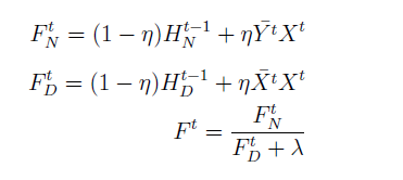
The main aim of MOSSE tracker is to learn a correlation filter that minimizes the squared error between convolution output (image patch \(x^{j}\) and the filter \(f\) and the expected output \(y^{j}\). \($x^{j}\),\(y^{j}\),\(f\) have spatial size of \(M \times N\) and depth of 1 since we are using grayscale images. Such a filter can be learnt by minimizing the following cost function \(\epsilon = \sum_{j=1}^{N} || f * x^{j} - y^{j}||^{2}\) \(x^{j}\) are the input patches extracted from frames \(j = 1…N\) for training. \(y^{j}\) are the 2D gaussian labels with peak centered on the target. Solving the problem in frequency domain helps us in exploiting the computational efficiency of the FFT. The problem can be reformulated in the frequency domain as. \begin{eqnarray} \min\limits_{F}\sum_{j=1}^{N} ||F \odot X^{j} - Y^{j}||^{2} \end{eqnarray} where \(\odot\) denotes element wise product. \(y^{j}\) and \(x^{j}\) are the FFT of image patch \(x^{j}\) and gaussian label \(y^{j}\). We can obtain a closed form solution for this minimization problem by taking derivative of equation w.r.t. F. The solution is given by \begin{equation} F = \frac{\sum_{j=1}^{N} \bar{Y^{j}}X^{j}}{\sum_{j=1}^{N} \bar{X^{j}}X^{j}} \end{equation} It was observed that an exact filter \(F\) trained on one image will almost always overfit that image. When applied to a new image, that filter will often fail. So a regularization step was proposed where \(\bar{X^{j}}X^{j}\) was replaced by \(\bar{X^{j}}X^{j}+\lambda\) where \(\lambda\) is the regularization parameter. The new filter is given by \begin{equation} F = \frac{\sum_{j=1}^{N} \bar{Y^{j}}X^{j}}{\sum_{j=1}^{N} \bar{X^{j}}X^{j} + \lambda} \end{equation} We need to adapt the filter to reflect changes in target appearance, rotation, scale, pose and lighting conditions. Moving average can be used for this purpose. The tracker is updated according to the following rule

\(F^{t}\)N and \(F^{t}\)D are the numerator and denominator of filter \(F^{t}\) where \(t\) denotes the frame number. \(\eta\) is the learning rate which assigns weightage to recent an previous frames. In the original implementation, \(\eta = 0.125\) was used which allows the filter to quickly adapt to appearance changes while still maintaining a robust filter.

Hierarchical Convolutional Features Tracker

MOSSE tracker learns a minimum output sum of squared error filter over luminance channel for fast visual tracking. It was observed that using feature representations like HOG instead of raw pixels may further improve the accuracy. HCF uses a combination of features extracted from different layers of CNNs as target representations may further improve accuracy. These features exploit semantics and fine-grained details to simultaneously handle large appearance variations and avoid drifting. HCF tries to learn multiple correlation filters using deep features from CNNs as opposed to only one single filter by existing approaches. We discuss HCF tracker in this section.

The aim of HCF tracker is to learn a correlation filter \(f\) that is best able to discriminate between the target object and the background pixels. It uses features extracted from different layers of VGGNet to learn such a filter. Let \(x\) denote VGGNet feature vector of dimension \(M \times N \times D\). We resize all the extracted features to a single size using bilinear interpolation. We learn such a filter by minimizing a loss function similar to that of MOSSE tracker. The important difference is the inclusion of more number of feature channels. The loss function is given by

\begin{eqnarray} \label{hcfProblem} \epsilon = \sum_{m,n} ||f \odot x_{m,n} -y_{m,n}||^{2} + \lambda||f||_{2}^{2} \end{eqnarray}

Here \(\lambda >0\) is the regularization parameter. \(y\) is the generated Gaussian label of size MxN which serves as the regression target. \(f\) is filter of dimensions of \(M \times N \times D\) which we are trying to learn by minimizing equation 2.8. \(f \odot x_{m,n}\) denotes inner product between the feature vector and the filter. The resultant inner product is summed over the feature depth to produce a single channel output i.e. \( f \odot x_{m,n} = \sum_{i=1}^{D} f_{m,n,d}^{T}x_{m,n,d}\). The closed form solution of equation 2.8 in frequency domain is given by

\begin{equation} F = (X^{H}X + \lambda I)^{-1}X^{H}Y \end{equation}

where \(X^{H}\) is the Hermitian transpose i.e. \(X^{H} = (X)^{T}\), and \(X^{}\) is the complex conjugate of X. The use of closed form solution in a real time setting is infeasible. A simpler solution was proved by Henriques et al. by exploiting useful properties of circulant matrices. With this assumption, the minimization problem has a solution similar to that of MOSSE tracker.

HCF features and response maps]{The features extracted from third, fourth and fifth convolutional layers from VGGNet are used to represent the target(left).The response map for different layers is shown(right).

\begin{equation} F^{d} = \frac{Y \odot \bar{X}^{d}}{\sum_{i=1}^{D}X^{i}\odot \bar{X}^{i} + \lambda} \end{equation}

The \(\odot\) refers to element wise product. All the capital letters denote the frequency domain counterparts of the variables. \subsection{Detection and filter update} The correlation response \(R \)can again be computed using the following formula: \begin{equation} R = \mathcal{F}^{-1}(\sum_{i = 1}^{D} F^{i} \odot \bar{Z}^{i}) \end{equation} \(Z^{i}\) denotes the features extracted from image patch in the next frame. The response \(R\) is of dimension MxN. We can obtain the predicted target position by finding the location of maximum value of \(R\). We need to adapt the filter model to account for changes in illumination, scale and target pose. We use a moving average model (similar to MOSSE tracker) given by the following equations:

\begin{eqnarray} A_{i}^{d} = (1-\eta)*A_{i-1}^{d} + \eta Y \odot \bar{X}^{d} \end{eqnarray}

\begin{eqnarray} B_{i}^{d} = (1-\eta)*B_{i-1}^{d} + \eta \sum_{i=1}^{D} X_{i}\bar{X}^{i} \end{eqnarray} \begin{eqnarray} F^{d} = \frac{A_{i}^{d}}{ B_{i}^{d} + \lambda } \end{eqnarray}

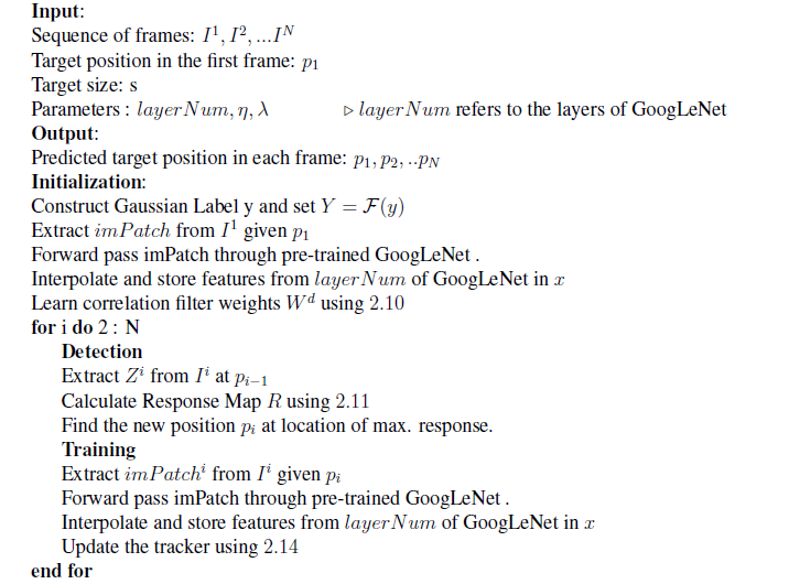
Here \(A^{d}\) and \(B^{d}\) are the numerator and denominator of \(F^{d}_{i-1}\) where \(d\) denotes the filter depth and \(i\) is the frame number. In this thesis, we have modified the HCF tracker to use a combination of CNN features extracted from different inception modules of GoogLeNet. We believe that this will enhance the computational efficiency with little effect on tracking accuracy. An algorithm highlighting the main steps is given below.