SRDCF-for-Object-Tracking
Spatially Regularized Correlation Filters
In this post I discuss the basics of the SRDCF framework. In most standard DCF approaches like MOSSE, the size of target search region used for training the classifier is limited. A naive increase in search region may lead to more emphasis on background instead of the target. This may hamper the discriminative power of the learned filter. To alleviate this problem, people have integrated deep features with the spatially regularized model. This approach lead to significant increase in performance.
Let \(x^{k}\) be one of the extracted feature map with spatial size of \(M \times N\) and depth \(d\). This feature map is generated by passing a cropped image containing the target object through a CNN. The cropped image includes the target region and some portion of background information also. In the original implementation, HOG features extracted from the cropped image were used modelling the target object. Let \(y^{k}\) be the corresponding target label of the generated feature map. A Gaussian function is used for generating this target label of spatial size \(M \times N\). Let \(f\) denote the learnt filter of spatial size \(M \times N\) and depth \(d\), where \(d\) is the number of feature maps. The desired filter \(f\) was obtained by minimizing the following cost function,
\begin{eqnarray} \epsilon = \sum_{m,n} || R_{m,n} -y_{m,n}||^{2} + \sum_{l=1}^{d}\lambda||w \cdot f^{l}||_{2}^{2} \end{eqnarray}
where \(\lambda > 0\) is the regularization parameter used to overcome overfitting. \(w\) refers to spatially regularized weights which have lower values around the target and have higher values as we move away from the target. The weights are generated using the function \(w = \mu + (m/P)^{2} + (n/Q)^{2}\) where P and Q are the size of the image patch and \(\mu\) = 0.1 and \(\eta\) = 3 are parameters.This strategy penalizes the background pixels and gives more emphasis on the target. A comparison of typical filters learnt using DCF and SRDCF approach is given in the below image.
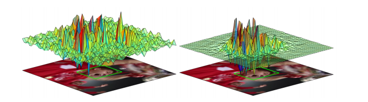
Comparison of the standard DCF (left) and the SRDCF (right). DCF has large filter coefficients residing in the background while SRDCF has peaks only near the target region. This is because filter coefficients further away from the target are penalized.
After obtaining the desired filters we can calculate the response \(R\) at \(M \times N\) spatial locations using the formula \begin{equation} R = \mathcal{F}^{-1}(\sum_{i = 1}^{d} F^{i} \odot \bar{X}^{i}) \end{equation} Here the symbols in capital are the fourier transforms of the original variables. The location of maximum response is the location of target object.
Dimensionality Reduction using PCA
One possibility may be to use features extracted from different layers of GoogLeNet for modelling the target object.The feature depths ranges from 512 to 1024 with spatial sizes varying from 28x28 to 7x7. The direct use of these higher dimensional features leads to high computational demand. In this section I introduce PCA which can be used for reducing the dimensions of extracted features from GoogLeNet. We use this technique in for visualizing the extracted features
Idea behind PCA
The basic idea behind principal component analysis is to find a new set of basis vectors which captures the direction of largest variations.The new basis vectors can provide us new insights regarding the data.
A figure illustrating this concept is given below. The data was first expressed in conventionally used coordinate system with X and Y axis as the basis vector. It can be observed that if the coordinate system is rotated then we can capture significant information about the data by using just one basis vector. The mathematical procedure for determining the new set of basis vectors obtained by rotating the initial basis is discussed below.

We can observe that basis vectors X\(‘\) and Y\(‘\) are better representatives of the data set than X and Y. Most of the data variation is along the X\(‘\) axis. So we can safely ignore Y\(‘\) axis without much loss of information.
Determining the new basis
Let X be a data vector. We need to find a vector P which can be geometrically thought as a rotation and stretch that provides a new representation for the data set i.e. \(PX = Y\). P acts as rotation needed to align the initial basis with the axis of maximal variance. Y is referred as the principal component of X. We want the covariance matrix \(C_{Y}\) to be a diagonal matrix. This will help us in minimizing the redundancy and decorrelate the variables. Rewriting the covariance \(C_{Y}\) in terms of PX we get the following.
\begin{aligned}
C_{Y} & = \frac{YY^{T}}{N} = \frac{(PX)(PX)^{T}}{N}
= \frac{PXX^{T}P^{T}}{N}
= P(\frac{XX^{T}}{N})P^{T}
= PC_{x}P^{T}
\end{aligned}
\begin{equation} C_{Y} = PC_{x}P^{T} \end{equation} We can use a result from linear algebra which states that any symmetric matrix A is diagonalized by an orthogonal matrix of its eigenvectors. Now we select \(P\) to be a matrix where each row \(p_{i}\) is an eigenvector of \(C_{X}\). Hence we can conclude that the principal components of X are the eigenvectors of covariance matrix \(C_{X}\). The eigenvectors \(v\) of \(C_{X}\) can be calculated using the following formula \begin{eqnarray} V^{-1}C_{X}V = D \end{eqnarray} where the columns of V are the eigenvectors \(v\), and D holds the eigenvalues \(\lambda\) in its diagonal. The eigen vectors with higher eigen values contain the most information about the data. We refer the reader to for more details and insights regarding PCA.
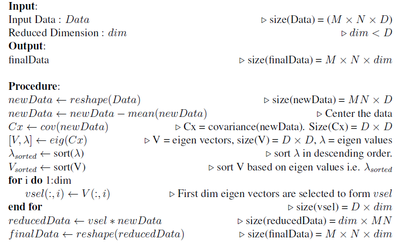
The following steps can be applied on the extracted features to reduce its dimensionality.