Betting amidst uncertainty

Life is uncertain, unpredictable and rife with randomness. Sometimes our well intentioned and best thought out decisions can go badly wrong. This fact isn’t as clear when we are younger, probably because we haven’t seen things fall apart. As we grow older and more experienced, the pollyanish young man is replaced with a bitter and extremely cautious old man, afraid to take any risks. There’s a middle path between extreme caution and irrational exuberance. This path, guided by logic, allows one to cautiously take risks.

The benefits of logical risk taking are not immediately obvious. It seems to be an abstract puzzle that maybe of interests only to mathematicians. I came across a beautiful betting game by Victor Haghani et al. (formerly associated with LTCM) that shows the practical utility of reason over intuition.

The objective of the game is to maximize the amount available to the user. The user is initially allocated $25. He has to predict Head/Tails and he can bet any amount he likes. If the guess is correct, he wins the allocated amount whereas if he is wrong, he loses the bet amount. The user can bet as many times as he likes. The only constraint is the time [5 minutes]. The interesting part about the game is that the coin is biased. The probability of heads is 0.6 whereas the probability of tails is 0.4. The biased nature of the coin is actually a blessing in disguise [more on this later]. The original implementation of the game is available here. I found the implementation to be a bit slow and less customizable. So, I reproduced the game for my personal experimentation.

Bidding Game

1. Click on Start to accept the game settings (defaults to 60-40 heads/tails probability).
2. Input amount that you wish to bid.
3. Select either Head/Tail.

Hint: It's easy to at-least end up with $200.

Available Amount: $25

Bid Amount:

Time remaining: 05:00

Game Settings

Win Return:
Lose Return:
Win Probability:

Win Probability: %

Win Return:

Lose Return:

I enjoy playing this game because it highlights some of our common behavioral biases. Behavioral economists like Daniel Kahneman have written extensively about these biases. While playing this game, people may follow prey to the following biases:

• Illusion of control
  In the context of this game, people may feel that if heads has occurred 5 times then tails is more likely to follow. This is not true, since every coin toss is an independent event.
• Anchoring
  Let's say one starts by betting $5 initially (total available amount=$25). When the total available amount increases to $100, he shouldn't be still anchored to his original amount (i.e. $5). Such a bet is demonstrably sub-optimal.
• Outcome Bias
  Let's say one has (reasonably) decided to always bet heads. After a string of tails, one shouldn't change their decision and start randomly betting tails. One shouldn't evaluate their decision based on the outcome. A string of tails is unlikely but can occur. Bad outcomes don't make the decision to predict heads incorrect.

The questions of calculated risk-taking have already been answered comprehensively by economists. Dr. Robert Merton and Dr. John Kelly have done seminal work in this area. Merton Share and Kelly Criterion can be used as a framework to think about risks and possibly take better decisions amidst uncertainties. As someone unfamiliar with economics, finance, and probability, I was unfamiliar with these techniques. (I am fond of linear algebra and calculus but dislike probability.)

Depending on the time that one spends on the problem, one can come up with multiple methods of betting. Among these methods, perhaps two approaches are the most intuitively appealing (at-least for me)

• Constant bets
At the beginning of the game, we decide what amount we are going to bet and stick with it throughout the game.
• Fractional betting
We always bet a fraction of the current available amount i.e. if we have $x, we always bet \($fx\) (where f is the fraction, like 0.1, 0.9 etc.)

Since in this experiment, heads is more likely than tails, we always bet heads. I must admit when one actually plays the game, one is tempted to bet tails after a string of heads. However, this isn't optimal.

Returns of constant betting

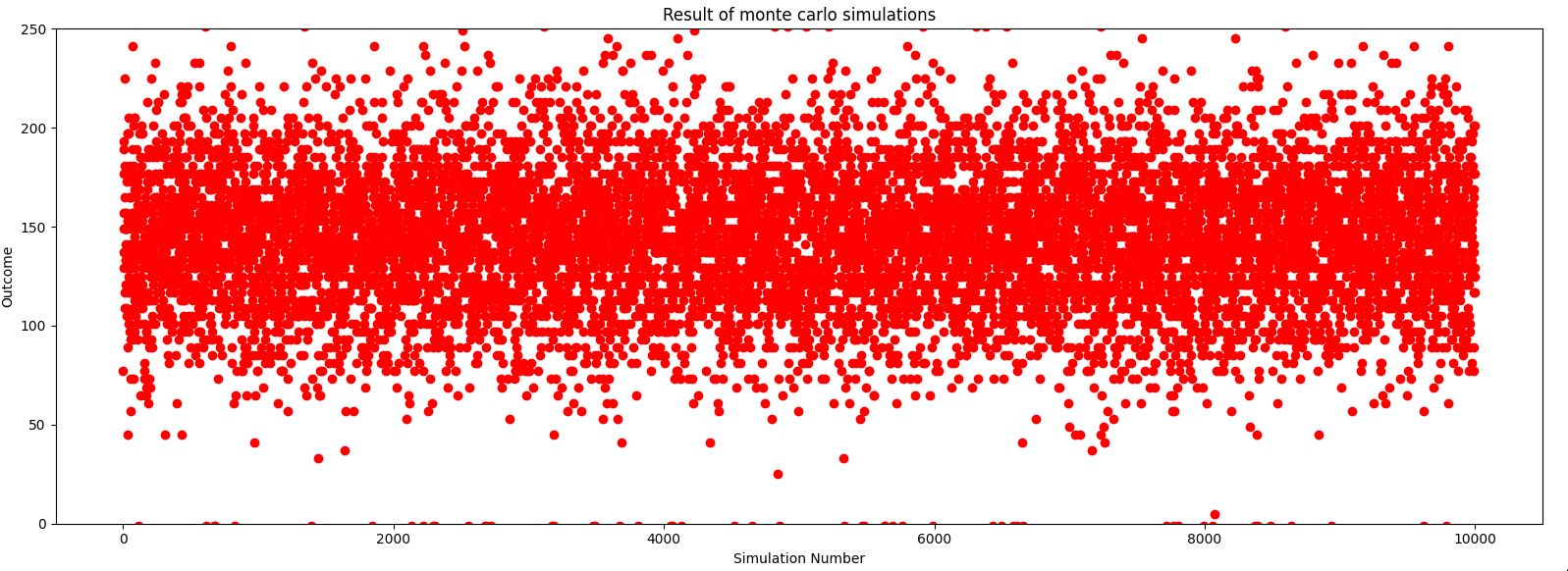
A risk averse person may like the idea of betting a fixed amount. Betting a fixed amount at every turn limits surprises and increases endurance. For example, if a risk averse person decides to always bet $1, he's extremely unlikely to end up with 0 balance. We can imagine the game as a Bernoulli trial. A person betting $1 can go bankrupt only if he loses the toss 25 times consecutively. Such an outcome is almost impossible 0.4²⁵ ~ 0.

It's quite complicated to exactly calculate what is the outcome of betting decisions mathematically. Fortunately, simple Monte Carlo simulations can be used to obtain a close estimate of the expected amounts and probabilities. In the following discussion, I have made the following assumptions

1. Maximum payout clipped to $250 This assumption helps makes sure that the estimate expected value is reasonable. Without such an assumption, the expected value will be close to ∞. If one considers the skewed distribution of returns, it's easy to see why this happens. There's a miniscule chance that the user is successful all the time. If one's fortune is so good, the expected payout will be $25*(2³⁰⁰) ~ 1.42*10²⁵.
2. Maximum number of bets that the user is allowed to make = 300 The game has a time constraint of 5 minutes ~ 300s. Even when the user makes a bet without any thought, he's unlikely to make more than 300 bets.

I ran 10 thousand monte carlo trials. In each trial, the user bet a constant amount. The trial ends if the user goes bankrupt or he makes 300 bets. The final amount available with the user is the outcome of each trial. At the end of the trial, we assign each outcome into 10 equidistant buckets ranging from $0 to $250. The probability of each bucket can be estimated by the number of trials in the bucket divided by the total number of monte carlo trials (10k). A typical monte carlo simulation is visualized below.

Each dot in this plot depicts the final amount available to the user at the end of a trial. It was assumed here that the user bets $2 irrespective of the available amount. The trial ends if he hits maximum payout ($250) or he's bankrupt. In the plot, it can be seen that very few trials end in bankruptcy.

Google Colab Notebook for replicating the results is available here.

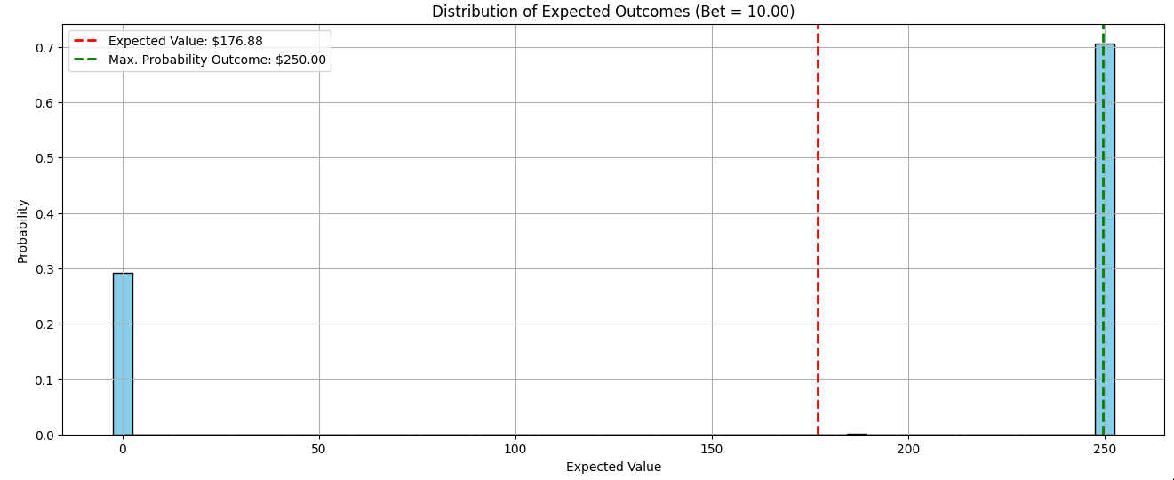
Distribution of outcomes for fixed betting strategy

The following plots show the probability of ending with different amounts for a fixed betting strategy. On the X-axis is the expected value and on the Y-axis is the probability. The expected value is plotted with a red line while the maximum probability outcome is depicted in green. Expected value was estimated by taking the weighted mean of probability and amounts. The Max. Probability Outcome refers to the amount that has the maximum chance of occurring.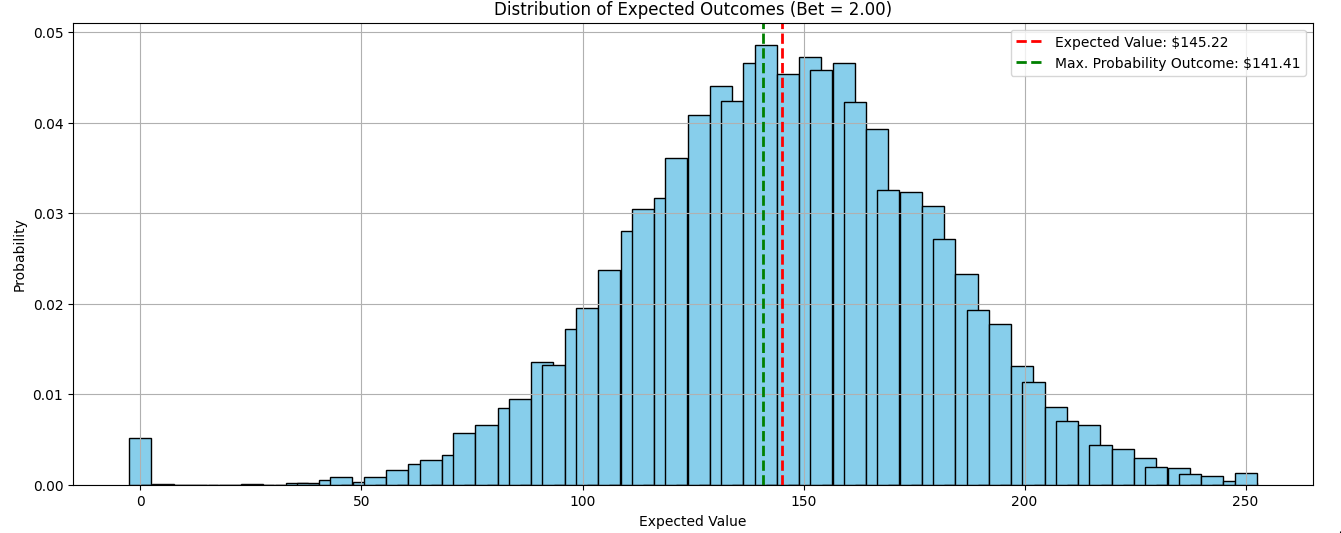

The left plot assumes that the user always bets $2 while right plot assumes that user always bets $10. In case the user bets $2, we can observe that the probability of ending with $0 is less than 1%. The probability of getting $250 is even lower (less than 1%).In contrast, if the user bets $10, the probability of obtaining $250 is significantly higher (around 70%). The downside is that the probability of total ruin is also high (around 30%).

Variation of outcomes for different constant bet strategies

I was curious to see what is the optimal amount that maximizes the expected value for constant bet strategy. So, I ran simulations for different fixed amounts. The results are shown in the plot below.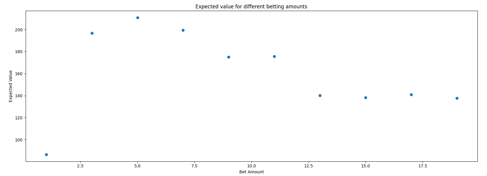

Each dot in this plot depicts the expected amount for a fixed amount betting strategy. One can observe that the expected value increases till $5 and starts decreasing subsequently. The risk of ruin is more than the gains while betting an amount greater than $5.

Returns of fractional betting

The downside of constant betting strategy is that it isn't adaptive. It keeps betting the same amount regardless of the available amount. Betting $5 when total balance is $25 is sensible while betting $5 when the balance is $100, is irrationally cautious. In contrast to the constant betting strategy, betting a fraction of the current available amount is adaptive and opens a path for better returns. The question of what fraction is optimal can be decided by the Kelly criterion.

Let \(f\) denote the fraction that we bet, \(p\) denote the probability of success and \(b\) be the proportion that we get, then as per Kelly criterion, $$f = p - \frac{(1-p)}{b}$$ In our case, \( p = 0.6 \) and \( b \) is 1 (since we only win the amount that we have bet). When we substitute these values, the optimal fraction comes out to be \( 0.6 - \frac{0.4}{1} = 0.2 \). Kelly Criterion is very popular in finance circles because it assures that there is no other betting strategy that maximizes the wealth in a shorter time. However, the strategy assumes that there are no limits on the maximum number of bets. This assumption is unrealistic. In real life, one can only make a finite number of bets. If a string of bad luck leads to huge losses, it may take a long time to recover.

Distribution of outcomes for different betting fractions

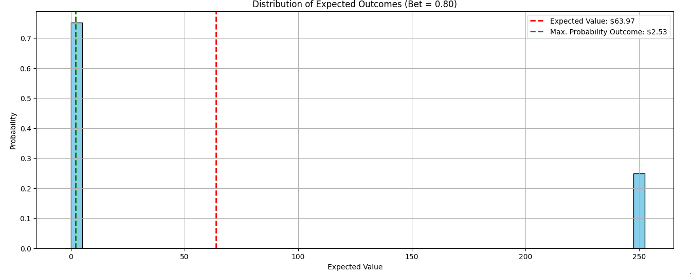
The following plots show the probability of ending with different amounts for a strategy that bets a fraction of the available amount. The axis labels and legend follow the earlier defined conventions.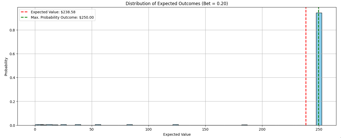

The left plot assumes that the user always bets 20% of the available amount while right plot assumes that user always bets 80%. We can observe that the expected value for 20% bet is $238.5 while it reduces to $63.9 for 80% bet. We can also observe that the probability of bankruptcy increases to around 25% for the 80% betting case. In contrast, the probability of bankruptcy is almost 0 for 20% case.

Variation of expected outcome for different constant bet strategies

As discussed earlier, according to the Kelly criterion the optimal betting fraction that maximizes the available amount is 0.2. So, we expect the expected values to increase as the betting fraction increases from 0 to 0.2 and subsequently start decreasing. The plot below tells a different tale. The optimal fraction seems to be 0.1 of the available amount!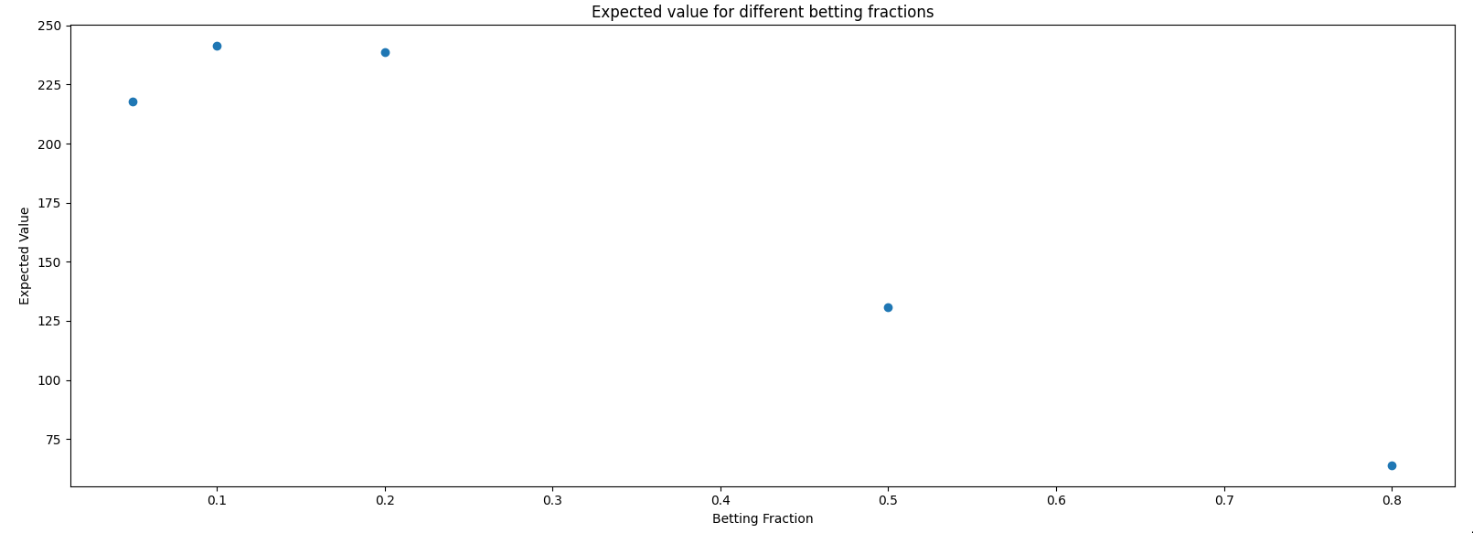

Each dot in this plot depicts the expected amount for a fractional amount betting strategy. One can observe that the expected value increases sharply increases till 0.1, plateaus till 0.2 and starts decreasing subsequently.

Resolving the discrepancy

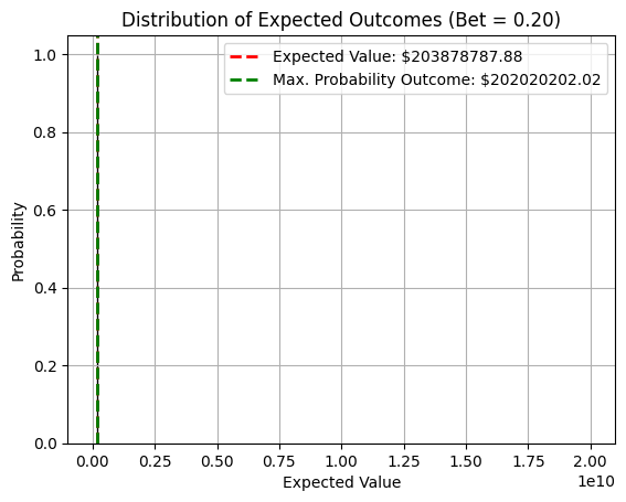
One of the assumptions that we made earlier during the monte carlo simulations was that the maximum payout is $250. This capping of maximum gain hurts when the betting fraction is 0.2. Without such an artificial limit, higher payouts can happen. To substantiate this point, I did two simulations where the max. payout limit was raised to 20 billion. In the plot below, we can clearly see that

The left plot shows the distribution when the user bets 10% of the available amount while right plot assumes that user always bets 20%. The maximum payout has been raised to 20 billion. The expected value for 10% betting scenario is 202 million while the expected value for 20% scenario is 203 million. This shows that the Kelly betting fraction is optimal without any artificial constraints.

An alternative way to resolve the discrepancy is to look at the simple proof of Kelly Criterion. The geometric rate of growth is given by $$ r = (1 + fb)^q (1 - fa)^p $$ The betting fraction \(f\) is obtained by taking the derivative and equating it to 0. In our case, the above formula for geometric rate of growth is invalid because of the maximum payout $250. $$ r = max( (1 + fb)^q (1 - fa)^p, M) $$ where the maximum growth is clipped to some value \(M\). The modified equation is non-differentiable, so we cannot take derivative. Monte Carlo simulations have to suffice to obtain estimates in such cases.

Conclusion

Sometimes I imagine our lives to be Monte Carlo trials. Each of us calculates and tries to accomplish our goals. Unfortunately, even our best decisions which have high probability of success (theoretically) can go wrong. The ultimate outcomes is beyond our control. A string of bad luck may break our will and convince us that logic and discipline are useless. On the other hand, good luck can engender within us false bravado. In both scenarios, it is wise to remain level headed and act logically. Only while acting logically, we are guaranteed to be asymptotically optimal.