An interesting pattern in the final fully connected layer weights

TL;DR
I have written a more formal summary of my findings in here.
Github: https://github.com/sidml/interpret-fc-layer
You can replicate my experiment results by running the notebooks in git repo or by running this Kaggle Notebook for fitting ALD and this for visualizing the internal split.
The results of fitting ALD to FC weights are here and visualization of the most discriminative neurons using Smooth GramCam++ is here.

Motivation

Like everyone else, I have struggled to interpret the predictions generated from neural networks. Sometimes networks fail on the most trivial of tasks and sometimes they succeed on the hardest. I have encountered similar difficulty while working with images, pointcloud data, text and even audio data. The interpretability of neural network predictions remains difficult regardless of the model architecture and input modality. I have tried in vain to formulate explanations about the failure cases for specific architectures and datasets. I haven’t been able to find theoretical backing or broad applicability of my explanations so I have refrained from posting about them till now.
Recently while reading about policy gradient methods in reinforcement learning, I thought of a possible connection between the current supervised learning paradigm and offline policy gradient RL. This observation allowed me to make a prediction regarding the distribution of weights in the final fully connected layer. I didn’t have high hopes but when I looked deeper, I observed that the weights of pre-trained ImageNet models indeed seem to closely follow a particular distribution, namely Asymmetric Laplace Distribution.

A thought experiment

Let’s say we have a dataset of images of cats & dogs that we want to classify. The straightforward way is to train a neural network using Cross Entropy Loss [CE Loss]. Comparing with RL, we can also think about the CE loss as a reward signal. If the network is misclassifying the images, then the reward will be low [i.e. loss will be high] and if it’s doing good, then reward will be high [i.e. loss will be low]. Next I wondered what is the counterpart of policy in SL ? In RL, policy roughly refers to the action (a_t) taken by the model in a particular state (s_t). The policy is learnt in RL. It’s a function of network parameter theta [so in RL,the notation $\pi_{theta}$ is commonly used]. Next i thought, what is the policy in SL case and how are we learning it?
In SL, the action is the classification of an image as cat/dog and the state (s_t) is the current input image. So SL policy can be thought as the possibility of selecting cat/dog (a_t) given an image (s_t). It is obvious that this policy must be a function of network parameters [since that’s what we are trying to learn in SL case]. However in SL, we never explicitly use the policy in the loss calculation or in the gradient descent step. This made me curious about how can we train the network without explicitly formulating a policy in SL case ?

Connecting policy gradient with SL

In this section I will attempt to give a quick sketch of the connection while keeping the mathematical details to a minimum. I suggest reading my summary for a more formal treatment. In RL, the objective is to maximize the sum of discounted future rewards of an agent. In the policy gradient setting, this is achieved by maximizing the following objective: \begin{equation} J({\pi_\theta}) = E_{\tau \sim p_{\pi_\theta}(\tau)}\left[ \sum_{t=0}^T R(s_t, a_t) \right]. \label{eq:rl_objective} \end{equation} In the above equation, we are most concerned about $\theta$ and $\pi$. $\theta$ denotes the model parameters that decide the policy $\pi$. Also note that the trajectory $\tau$ is sampled from this learnt policy parameterized by $\theta$. Now coming back to SL, we can imagine the trajectory to be the batch sampling procedure. If you are not using some fancy data sampling technique like SMOTE or a weighted data sampler, then this trajectory should only be dependant on the dataset distribution. Based on the policy gradient formulation, $\tau$ is supposed to be sampled from $\pi_\theta$ [refer to this term $\tau \sim p_{\pi_\theta}$]. Since $\tau$ is a function of dataset distribution so we can conclude that $p_{\pi_\theta}$ must also be function of the dataset distribution. The gradient of the objective $J({\pi_\theta})$ with respect to $\theta$ is given by \begin{equation} \nabla J({\pi_\theta}) = E_{\tau \sim {\pi_\theta}}[(\sum_{t=1}^T \nabla log {\pi_\theta}(a_t,s_t))] (\sum_{t=1}^T r(s_t,a_t)] \label{eq:rl_grad_objective} \end{equation}

As you can see if we use gradient descent, then the policy makes an appearance here $\nabla log {\pi_\theta}(a_t,s_t))$. However we remarked earlier that the SL policy is solely dependant on our sampling procedure and definitely not on the network parameters. So during gradient descent, we must make sure that the policy doesn’t contribute. This can be simply achieved by setting it to some scalar value i.e $\nabla_{\theta} log {\pi_\theta}(a_t,s_t))$ is set to 1. If we do that then can see that $\theta$ must have been drawn from an exponential family of distributions of the form $exp(a*\theta+b)$, where $a$ and $b$ are some scalars. This distribution is called an asymmetric laplace distribution. In the formal summary I provide another way of motivating this particular distribution.

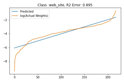
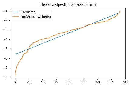
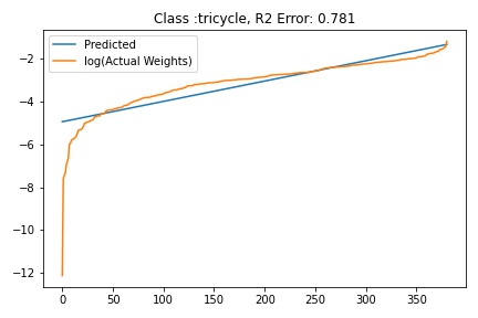
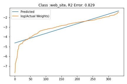
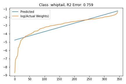
Fitting ALD to the final layer weights

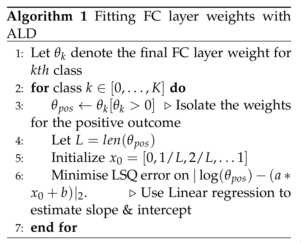
The next step is to fit ALD the final layer weights for all the classes. It is relatively straight forward to fit the distribution. I followed this approach. It is possible that there are better approaches to fit ALD that I am not aware of. If so, kindly let me know in the comments.

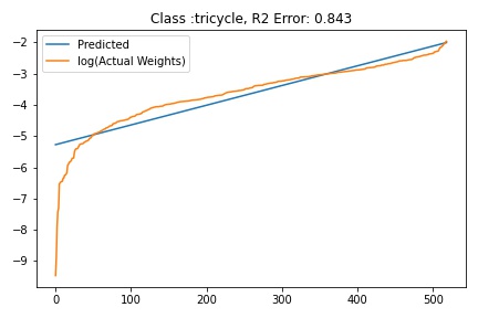
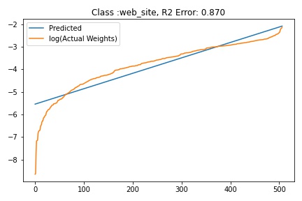
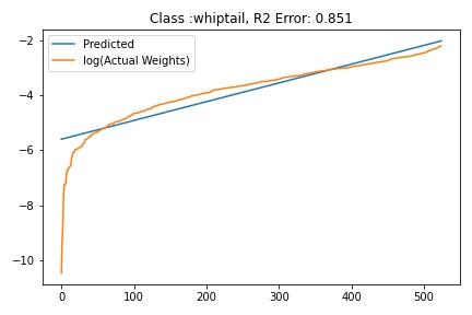
Results

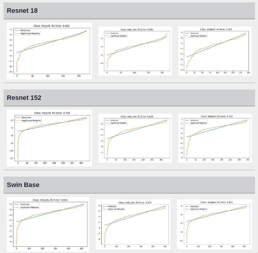
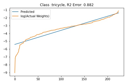
I tried to fit ALD to the FC layer of pre-trained models available on timm . Below you can the results for Swin, Resnet 18 and Resnet152. I selected these architectures in particular to show to show the wide applicability of the proposed fitting method. Resnet18 was selected as an example of a very small CNN based model, Resnet152 was selected to represent large CNN based models and Swin was chosen as a representative of the vision transformer class of models. Using the notebook you can verify similar results for other architectures as well. The only exceptions will be model architectures trained with custom sampling procedure that skews the dataset distribution. In such cases, the policy can be no longer assumed to follow the dataset distribution and thus ALD cannot be fitted.

Resnet 18

Resnet 152

Swin Base

Possible implications

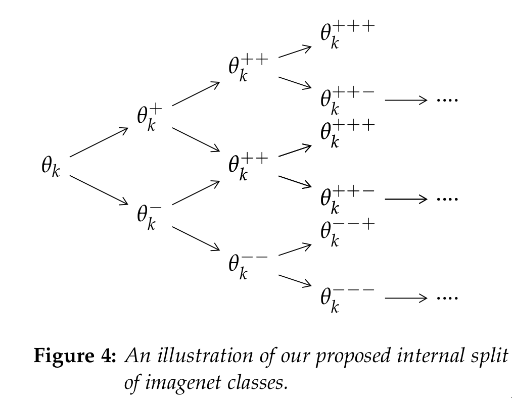While fitting ALD distributions to the FC layer weights for each class $\theta_k$, I observed a recursive pattern in the isolated weights. Let $\theta_k^+$ denote the weights for the positive sub-class [i.e. the possibility that the sample belong to class k] \& $\theta_k^-$ denote the weights for the negative class [i.e. the possibility that the sample is outside training set]. I hypothesize that $\theta_k^+$ and $\theta_k^-$ can be further sub-divided and fitted with ALD. An illustration of this idea is given in above figure. The proposed recursive partition of weights $\theta_k$ can help us isolate the most discriminative and most confusing feature according of the input image for the neural network. More specifically, let $\theta_k^{+++}$ denote the final tree node in the positive part after the proposed split of the weights $\theta_k$. Since these tree nodes were always encountered while maximizing the possibility of kth class, the associated neurons should activate on the most vital feature for the kth class. Similarly the terminal weights in the negative branch $\theta_k^{—}$ should encode the most confusing aspect for the kth class.

To verify this hypothesis, I used Smooth Grad-Cam ++ to highlight image regions associated with the most activated positive $\theta_k^{++..}$ and negative terminal $\theta_k^{–..}$ weights for the target class.

A visualization of the weights can be found in figure given below [It is a html page so the rendering is sometimes not correct. You may need to zoom a bit]. We applied our split method to identify the most important neurons in the final fully connected layer in Resnet34. The activation associated with only the most discriminative neurons at each stage were used for the visualization. In the figure, we report activations for each stage of the split for reference. For example: +2 & -2 refers to the positive and negative branches after the first split. We used this notation to avoid clutter. A more descriptive notation could be $\theta_k^{++}$ and $\theta_k^{–}$ as used earlier in the previous tree diagram.
In our experiments, we observed that it is difficult to interpret the activations of neurons from the intermediate stages. We found the activations in the terminal node easier for subjective interpretation. The visualizations were generated using images from validation set of ImageNet. More results can be found here.

Results on the tailed frog class from ImageNet.

Results on the American Lobster class from ImageNet.

Possible Applications

• Model robustness on test data
  If there is prior knowledge about the data distribution then it can be incorporated during the supervised learning stage by adjusting the policy gradient during loss calculation step. This process can be particularly useful for imbalanced datasets.
• Pruning the final fully connected layer
  If a prior distribution is known for the dataset then network weights which show high deviation from the prior distribution can be pruned away without hurting the model accuracy significantly.
• Explaining model outputs
  If the claim regarding recursive split of +ve & -ve templates holds, then the visualization of these templates perhaps using Smooth Grad-CAM & related methods, can help us get better insights into the model decision.

Importance of explainability & Prior Attempts

Traditional methods like Decision Trees and Rule based methods have high explanatory power but lag behind deep neural networks in performance. Nowadays it has become very easy to deploy which has led to their widespread usage. Hence I think the issue of interpretability and explainability has become even more pressing. Explainability is particularly important in high stake applications like autonomous driving and medical diagnosis. Aside from the practical benefit of explainable decisions [which should be a huge motivation imho], interpretable deep neural networks will help us in distilling out the important aspects of network architecture and training methodology. These insights will help us to develop a new class of explainable neural networks which will hopefully be more data efficient, have smaller number of neurons and be able to efficiently utilize inductive priors.
Currently popular neural networks are vastly over-parameterized, sometimes requiring millions of parameters to solve seemingly simple visual classification problems. This is a commonly accepted phenomenon but it is not intuitive. The natural world already has organisms like nematodes which display interesting behavioral patterns even though they have a very small number of neurons. The adaptability and robustness of such simple organisms in challenging environments points towards a gap in our understanding of neural networks.

Given the important of explanability, many methods have been proposed to understand neural network predictions. Attribution based methods & perturbation based methods are the two popular approaches that I am aware of. Attribution based methods aim at characterizing the response of neural networks by finding which parts of the network’s input are the most responsible for determining its output. These methods generally use backpropagation to track information from the network’s output back to its input, or an intermediate layer. Methods like GradCAM, and Guided Backprop are the most famous example of these kind of methods.
Approaches like RISE and Meaningful Perturbations belong to the perturbation family of methods. These methods perturb the inputs to the model and observe resultant changes to the output. Although these methods are interesting, they still have drawbacks. For example, methods like GradCAM may capture average network properties but may not be able to characterize intermediate activations, or sometimes the model parameters.

References:
^{_{Sutton, R.S., Barto, A.G. (2018). Reinforcement Learning: An Introduction, MIT Press.
Levine, S. (2017). Policy gradient introduction. Lecture slides, CS 294: Deep Reinforcement Learning, UC Berkeley.
Felix Marin. Difference of two exponential distribution. Mathematics Stack Exchange.
Omeiza, Daniel and Speakman, Skyler and Cintas, Celia and Weldermariam, Komminist. Smooth grad-cam++: An enhanced inference level visualization technique for deep convolutional neural network models. arXiv preprint arXiv:1908.01224.
Selvaraju, Ramprasaath R et al. Grad-cam: Visual explanations from deep networks via gradient-based localization. Proceedings of the IEEE international conference on computer vision.
Petsiuk, Vitali and Das, Abir and Saenko, Kate. Rise: Randomized input sampling for explanation of black-box models. arXiv preprint arXiv:1806.07421.
Ross Wightman. PyTorch Image Models. GitHub repository.}}